[ADVANCED] How Doodler works
See our journal manuscript for the most comprehensive explanation for how Doodler works
Citation: Buscombe, D., Goldstein, E.B., Sherwood, C.R., Bodine, C., Brown, J.A., Favela, J., Fitzpatrick, S., Kranenburg, C.J., Over, J.R., Ritchie, A.C. and Warrick, J.A., 2021. Human‐in‐the‐Loop Segmentation of Earth Surface Imagery. Earth and Space Science, p.e2021EA002085 https://doi.org/10.1029/2021EA002085
Overview#
Sparse annotation or 'doodling'#
It all begins with your inputs - doodles. This is what the subsequent list of operations are entirely based upon, together with some spatial logic and some assumptions regarding the types of 'features' to extract from imagery that would collectively best predict the classes.

Image standardization#
Doodler first standardizes the images, which means every pixel value is scaled to have a mean of zero and a variance of 1, or 'unit' variance. For the model, this ensures every image has a similar data distribution. It also acts like a 'white balance' filter for the image, enhancing color and contrast.
Feature extraction#
Doodler estimates a dense (i.e. per-pixel) label image from an input image and your sparse annotations or 'doodles'. It does this by first extracting image features in a prescribed way (i.e. the image features are extracted in the same way each time) and matching those features to classes using Machine Learning.
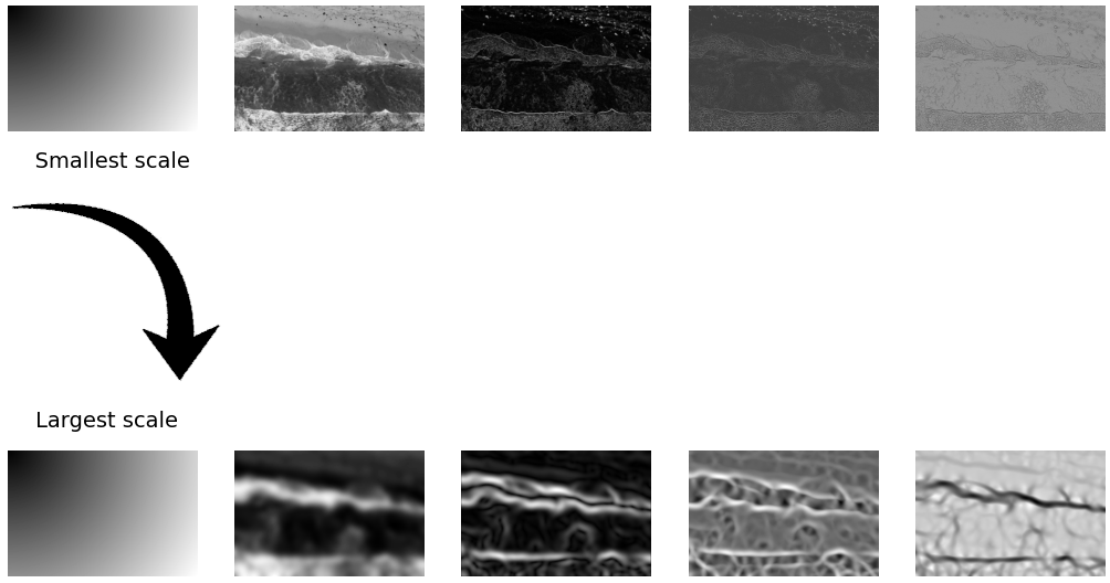
Doodler extracts a series of 2D feature maps from the standardized input imagery. From each sample image, 75 2D image feature maps are extracted (5 feature types, across 15 unique spatial scales)
The 5 extracted feature types are (from left to right in the image below):
- Relative location: the distance in pixels of each pixel to the image origin
- Intensity: Gaussian blur over a range of scales
- Edges: Sobel filter of the Gaussian blurred images
- Primary texture: Matrix of texture values extacted over a range of scales as the 1st eigenvalue of the Hessian Matrix
- Secondary texture: Matrix of texture values extacted over a range of scales as the 2nd eigenvalue of the Hessian Matrix
In the figure below, only the 5 feature maps extracted at the smallest and largest scales are shown for brevity:
Initial Pixel Classifier#
As stated above, Doodler extracts features from imagery, and pairs those extracted features with their class distinctions provided by you in the form of 'doodles'. How that pairing occurs is achieved using Machine Learning, or 'ML' for short. Doodler uses two particular types of ML. The first is called a 'Multilayer Perceptron', or MLP for short. The seond ML model we use is called a "CRF' and we'll talk about that later.
The first image is "doodled", and the program creates a MLP model that predicts the class of each pixel according to the distribution of features extracted from the vicinity of that pixel.
Those 2D features are then flattened to a 1D array of length M, and stack them N deep, where N is the number of individual 2D feature maps, such that the resulting feature stack is size MxN. Provided label annotations are provided at a subset, i, of the M locations, M_i, so the training data is the subset {MxN}_i. That training data is further subsampled by a user-defined factor, then used to train a MLP classifier.
Below is a graphic showing, for this particular sample image we are using in this example, how the trained MLP model is making decisions based on pairs of input features. Each of the 9 subplots shown depict a 'decision surface' for the two classes (water in blue and land in red) based on a pair of features. The colored markers show actual feature values extracted from image-feature-class pairings. As you can see, the MLP model can extrapolate a decision surface beyond the extents of the data, which is useful in situations when data is encountered with relatively unusual feature values.
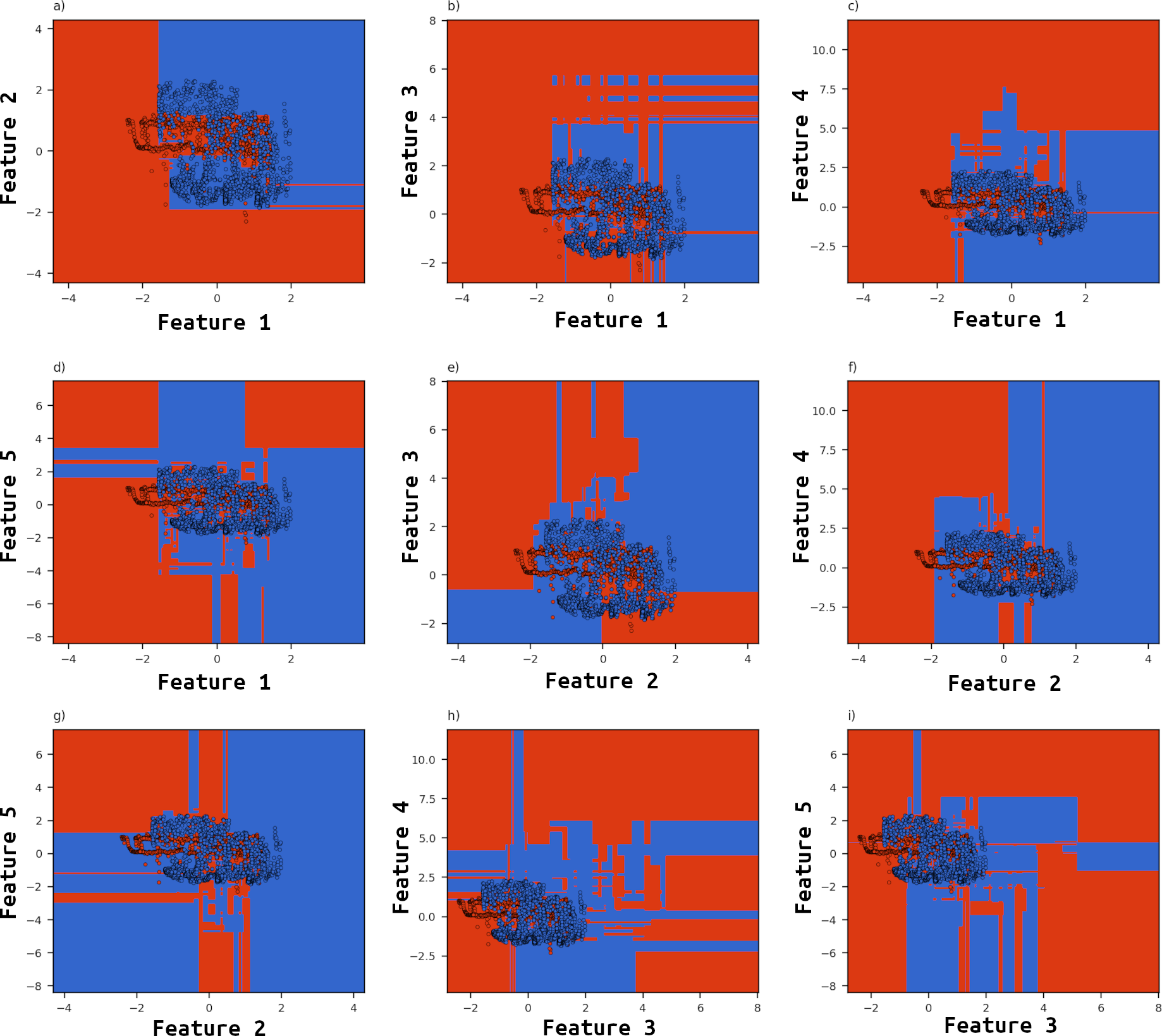
In reality, the MLP model does this on all 75 features and their respective combinations (2775 unique pairs of 75 features) simultaneously. It combines this information to predict a unique class (encoded as an integer value) for each pixel. The computations happen in 1D, i.e. on arrays of length MxN, which are then reshaped. Therefore the only spatial information used in prediction is that of the relative location feature maps.
Tip
The program adopts a strategy similar to that described by Buscombe and Ritchie (2018), in that a 'global' model trained on many samples is used to provide an initial segmentation on each sample image, then that initial segmentation is refined by a CRF, which operates on a task specific level. In Buscombe and Ritchie (2018), the model was a deep neural network trained in advance on large numbers of samples and labels. Here, the model is built as we go, building progressively from user inputs. Doodler uses a MLP as the baseline global model, and the CRF implementation is the same as that desribed by Buscombe and Ritchie (2018)
Spatial filtering of MLP predictions#
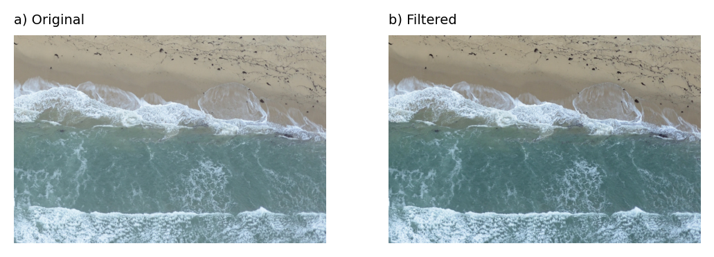
Each MLP prediction (a label matrix of integer values, each integer corresponding to a unique class). That corresponds to the left image in the figure below. You can see there is a lot of noise in the prediction; for example, and most notably, there are several small 'islands' of land in the water that are model errors. Therefore each label image is filtered using two complementary procedures that operate in the spatial domain.

The first filtering exercise (the outputs of which are labeled "b) Filtered" in the example figure above) operates on the one-hot encoded stack of labels. For each, pixel 'islands' less than a certain size are removed (filled in with the value of the surrounding area). Additionally, pixel 'holes' are also sealed (filled in with the value of the surrounding area). You can see in the example, by comparing a) and b) in the above figure, that many islands were removed in this process on this particular example.
The second filter then determines a 'null class' based on those pixels that are furthest away from similar classes. Those pixels occur at the transition areas between large contiguous regions of same-class. The process by which this is acheived is described in the figure below:
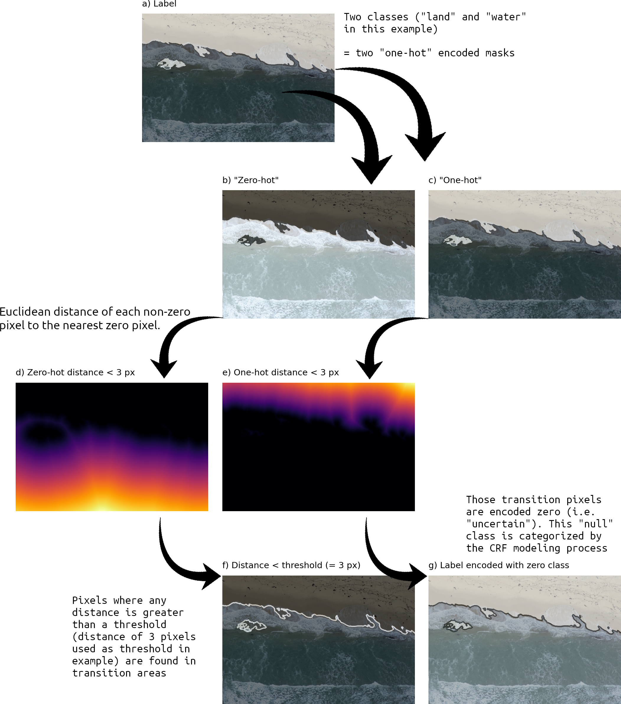
The intuition for 'zeroing' these pixels is to allow a further model, described below, to estimate the appropriate class values for pixels in those transition areas.
Conditional Random Field Modeling#
Tip
Already you can see how we are building a lot of robustness to natural variability:
- images are standardized
- Other measures are made to prevent model overfitting, such as downsampling
- Different types of image and location features are used and extracted at a variety of scales
- MLP outputs are filtered using relative spatial information
Next we'll go even further by making use of both global and local predictions.
The global predictions are provided by the MLP model. They are called 'global' because the model is built from all doodled images in a sequence.
The local predictions are provided by a different type of ML model, called a CRF, which is explained below.
That initial MLP provides an initial estimate of the entire label estimate, which is fed (with the original image) to a secondary post-processing model based on a fully connected Conditional Random Field model, or CRF for short. The CRF model refines the label image, using the MLP model output as priors that are refined to posteriors given the specific image. As such, the MLP model is treated as a initial model and the CRF model is for 'local' (i.e. image-specific) refinement.
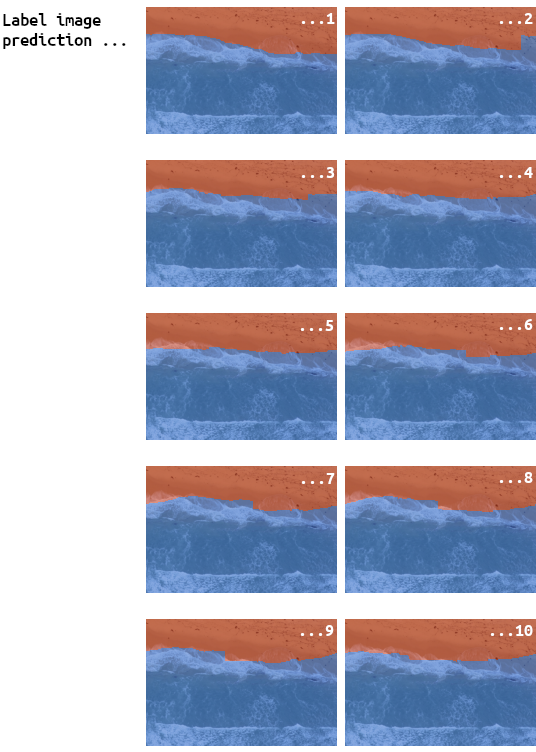
The CRF builds a model for the likelihood of the MLP-predicted labels based on the distributions of features it extracts from the imagery, and can reclassify pixels (it is intended to do so). Its feature extraction and decision making behavior is complex and governed by parameters. That prediction then is further refined by applying the model to numerous transformed versions of the image, making predictions, untransforming, and then averaging the stack of resulting predictions. This concept is called test-time-augmentation and is illustrated in the figure below as outputs from using 10 'test-time augmented' inputs:
Spatial filtering of CRF prediction#
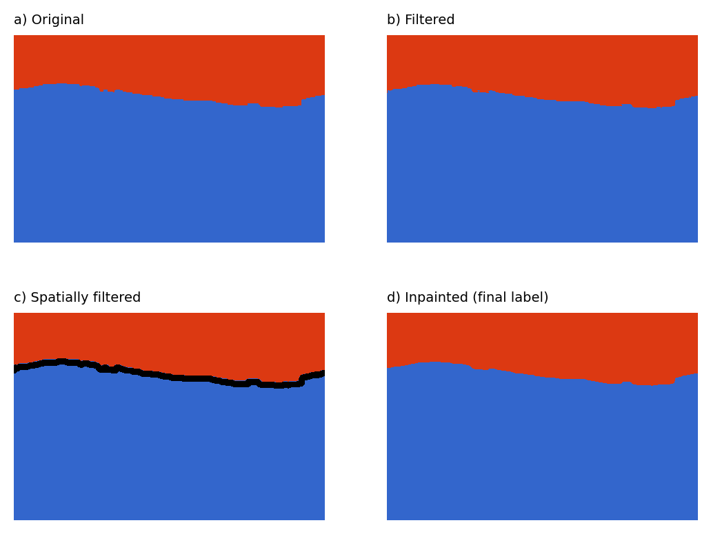
The label image that is the result of the above process is yet further filtered using the same two-part spatial procedure described above for the MLP model outputs. Usually, these procedures revert fewer pixel class values than the equivalent prior process on the MLP model outputs. The outputs are shown in 'b) and c)' in the figure below. A final additional step not used on MLP model outputs is to 'inpaint' the pixels in identified transition areas using nearest neighbor interpolation ('d)' in the figure below)
A final label image is then stored in disk:
